Drill down to nuScenes dataset (4/6)
in Tutorial with 0 comment
Drill down to nuScenes dataset (4/6)
in Tutorial with 0 comment

This is an in-depth article following the official tutorial. There are 6 official tutorials. Now this is can_bus_tutorial.ipynb, which is the fourth article. The link is: here

The six tutorials are as follows:

background

CAN bus expansion is additional information released in January 2020 after the first release of nuScenes in March 2019. These data can be used for tasks such as trajectory estimation, target detection and tracking.

CAN bus is used for communication between cars, including low-level messages about position, speed, acceleration, steering, lights, batteries, etc. In addition to the original data, it also provides some metadata, such as statistics of different message types. Please note that, CAN bus data is highly experimental. Some data may be redundant in different messages. Finally, the fragment information of the current driving route of the vehicle is also extracted.

preparation

Download dataset: you need to register first, and then enter the download page: https://www.nuscenes.org/download , find the CAN bus expansion, md5: 32ce964b131988c3ff6279731a516e6f, Click Asia to download, because aws s3 is officially used for storage. If the download is not smooth, please bring your own magic.

Extract the downloaded dataset to~/data_sets. The complete directory is /Users/lau/data_sets/nuscenes , this directory will be used later.

Reading Datasets

initialization

Start jupyter and create can_bus.ipynb

 from nuscenes.can_bus.can_bus_api import NuScenesCanBus nusc_can = NuScenesCanBus(dataroot='/Users/lau/data_sets/nuscenes')

Overview

Let's summarize all CAN bus messages and some basic statistics (minimum, maximum, average, standard deviation, etc.). We will select an arbitrary scenario for analysis.

 scene_name = 'scene-0001' nusc_can.print_all_message_stats(scene_name) #Output results { "ms_imu": [ "ms_imu", "pose", "steeranglefeedback", "vehicle_monitor", "zoe_veh_info", "zoesensors" ], "pose": [ "ms_imu", "pose", "steeranglefeedback", "vehicle_monitor", "zoe_veh_info", "zoesensors" ], "steeranglefeedback": [ "ms_imu", "pose", "steeranglefeedback", "vehicle_monitor", "zoe_veh_info", "zoesensors" ], "vehicle_monitor": [ "ms_imu", "pose", "steeranglefeedback", "vehicle_monitor", "zoe_veh_info", "zoesensors" ], "zoesensors": [ "ms_imu", "pose", "steeranglefeedback", "vehicle_monitor", "zoe_veh_info", "zoesensors" ], "zoe_veh_info": [ "ms_imu", "pose", "steeranglefeedback", "vehicle_monitor", "zoe_veh_info", "zoesensors" ] }

visualization

Next, we will plot the value of the CAN bus message over time.

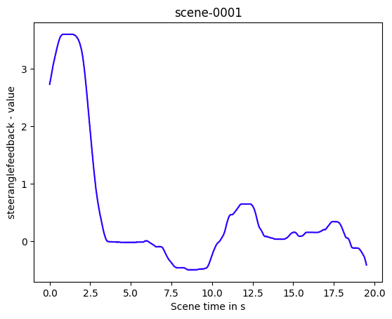
Take the steering angle feedback message as an example, use the README The Value keyword described in. The following figure shows the steering angle. It seems that the scene starts with a strong left turn, and then continues to basically go straight.

 message_name = 'steeranglefeedback' key_name = 'value' nusc_can.plot_message_data(scene_name,  message_name, key_name)
 2023-05-26T13:45:55.png

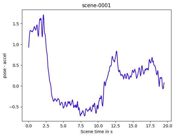
If the data we want to plot is multidimensional, we need to provide an additional parameter to select dimensions. Here we plot the acceleration along the horizontal dimension (y-axis). We can see that the initial acceleration is high.

 message_name = 'pose' key_name = 'accel' nusc_can.plot_message_data(scene_name,  message_name, key_name, dimension=1)
 2023-05-26T13:46:37.png

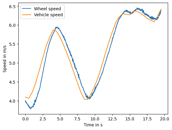
We can also obtain raw data and compare wheel speed with vehicle speed. Here we convert the wheel speed from revolutions per minute to meters per second, and the vehicle speed from kilometers per hour to meters per second. We can see that there is a small deviation between the velocities.

 import numpy as np import matplotlib.pyplot as plt # Retrieve raw data. wheel_speed = nusc_can.get_messages(scene_name, 'zoe_veh_info') wheel_speed = np.array([(m['utime'],  m['FL_wheel_speed']) for m in wheel_speed]) veh_speed = nusc_can.get_messages(scene_name, 'vehicle_monitor') veh_speed = np.array([(m['utime'],  m['vehicle_speed']) for m in veh_speed]) # Convert to m/s. radius = 0.305  # Known Zoe wheel radius in meters. circumference = 2 * np.pi * radius wheel_speed[:, 1] *= circumference / 60 veh_speed[:, 1] *= 1 / 3.6 # Normalize time. wheel_speed[:, 0] = (wheel_speed[:, 0] - wheel_speed[0, 0]) / 1e6 veh_speed[:, 0] = (veh_speed[:, 0] - veh_speed[0, 0]) / 1e6 plt.plot(wheel_speed[:, 0],  wheel_speed[:, 1]) plt.plot(veh_speed[:, 0],  veh_speed[:, 1]) plt.xlabel('Time in s') plt.ylabel('Speed in m/s') plt.legend(['Wheel speed', 'Vehicle speed']);
 2023-05-26T13:47:57.png

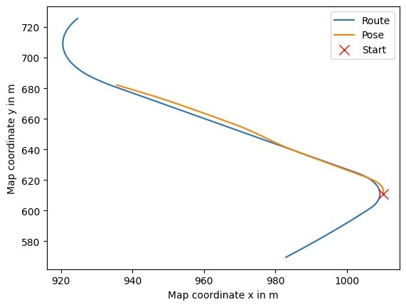
Now let's render the baseline of this scene. The blue line below shows the baseline that extends 50 meters beyond the start and end points of the scene. The orange line indicates the self driving attitude. To distinguish the starting point from the ending point, we mark the starting point with a red cross. We can see that there is a slight deviation between the actual attitude and the route.

 nusc_can.plot_baseline_route(scene_name)
 2023-05-26T13:48:45.png

error handling

Note that some scenes do not align well with the baseline alignment. This may be due to diversion or because human drivers do not follow the route. We calculate all misaligned routes by checking whether each self driving attitude is within 5 meters of the reference route.

 print(nusc_can.list_misaligned_routes())

In addition, few scenarios have no CAN bus data at all. Therefore, these scenes cannot be used.

 print(nusc_can.can_blacklist)

reference resources

Responses