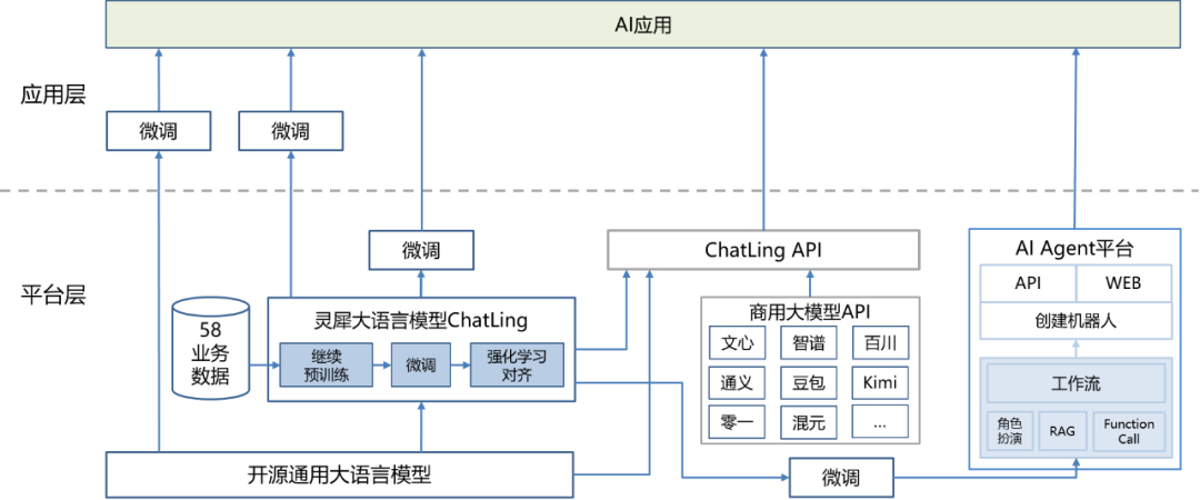
In 2023, big models will spring up like mushrooms. As an AI platform department, 58 local TEG AI Lab has closely followed the development pace of big language model technology, built a big language model platform, supported big language model training and reasoning deployment, and built a large vertical model of 58 local life service fields (real estate, recruitment, cars, yellow pages) based on the big language model platform Lingxi big language model（ ChatLing ）And supported the exploration and implementation of the business side's large model application. Lingxi big language model is better than open source general big language model and commercial general big language model in both open evaluation collection and actual application scenarios.

In the process of developing Lingxi large model, we have carried out extensive practice on the PEFT (Parameter Efficient Fine Tuning) of large model parameters. This paper systematically analyzes several commonly used large model parameter efficient fine tuning (PEFT) methods, and introduces the algorithm principle and application effect of each method in detail. First, this paper will describe the importance and basic concepts of efficient parameter tuning, and then briefly introduce the two PEFT methods, Adapter Tuning and Prefix Tuning, before LoRA tuning. Then this paper will introduce four efficient parameter methods, LoRA (Low Rank Adaptation), QLoRA (Quantized LoRA), AdaLoRA (Adaptive Low Rank Adapter), and SoRA (Sparse low rank adaptation) in detail. These methods are designed to reduce the amount of training parameters, reduce the cost of fine-tuning, while maintaining model performance. In addition, this paper will share the practical experience of fine tuning acceleration based on Unslow, and show the training acceleration effect and video memory occupancy reduction effect on different models and data sets. To sum up, this paper will share relevant technical analysis and practical experience from the perspectives of fine-tuning methods and training acceleration.

PEFT

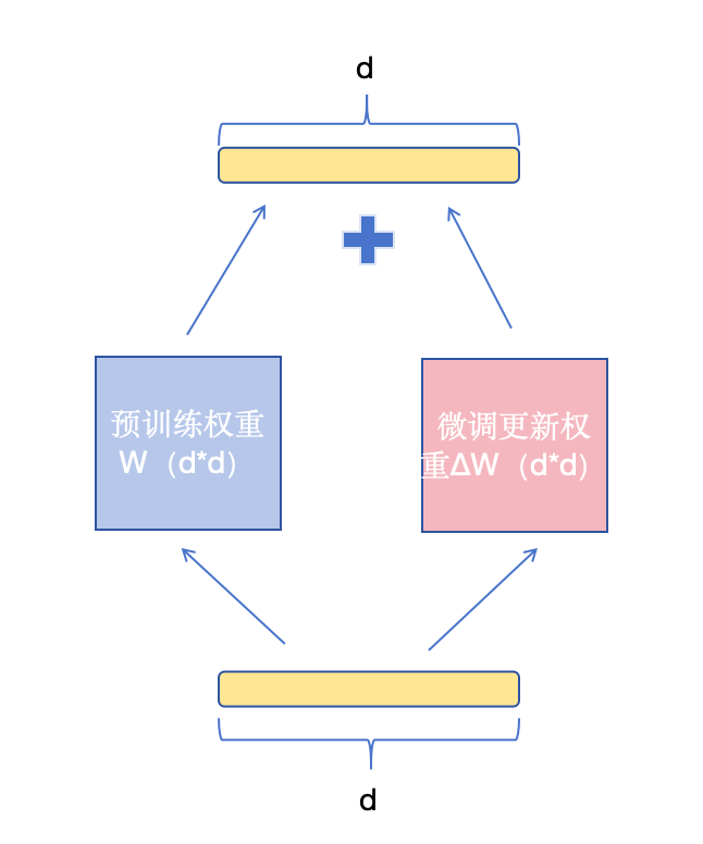
Since ChatGPT became popular, many manufacturers have devoted themselves to the R&D and application of AI large-scale language models. However, the high computing cost makes it difficult for many people to train a large language model from scratch. Therefore, since the era of Transformer and BERT, fine tuning technology has been favored because of its affinity to people. For business applications, the language model trained on a large number of corpora based on the open source model, and then fine tuned for specific business field data, this more cost-effective method seems to meet the needs of most companies at the current stage. Fine tuning technology refers to further training a trained model (pre training model) through specific downstream task data, so that the model can better adapt to the needs of specific tasks. As an efficient feature extractor, the pre training model can extract effective features based on the experience accumulated in previous training data, thus significantly improving the training effect and convergence speed of downstream tasks. Full parameter fine-tuning refers to updating all parameters of the pre training model during the training process of downstream tasks. As shown in the figure below, each parameter (d * d parameters) in the weight matrix should participate in the update during the fine-tuning process. However, for large-scale language models, traditional full parameter fine-tuning methods require extremely high computing resources and time costs. For example, recently released open source models such as LLaMA 3-70B, Qwen 1.5-110B and DeepSeek-V2 are too large for ordinary users to tolerate even fine tuning.

However, since the model has seen enough data and gained enough experience in the pre training stage, I just need to find a way to add an additional knowledge module to the model, so that this small module can adapt to my downstream tasks, and the model body can remain unchanged. This is called efficient parameter fine-tuning. This method can obviously reduce the amount of training parameters, reduce the cost of fine-tuning, and greatly improve the efficiency of fine-tuning. Next, this article will introduce several widely used efficient fine-tuning methods.

Adapter Tuning and Prefix Tuning

Adapter Tuning

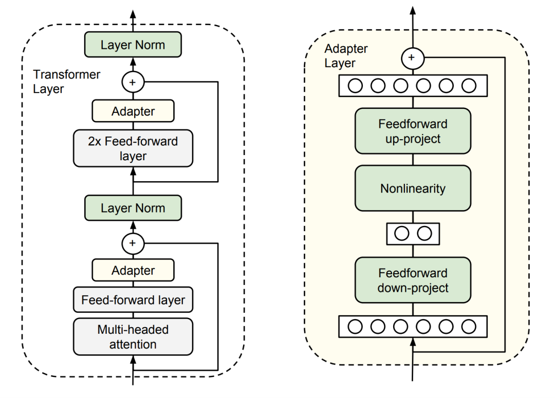
In 2019, Adapter Tuning will introduce Adapter into the NLP field as an alternative to full model tuning. The main structure of the adapter is shown in the figure below. The left side of the figure is a Transformer Layer structure, in which the Adapter is the "extra knowledge module" described above; On the right is the specific structure of Adatper. During fine tuning, all parameters except the adapter are frozen, which can effectively reduce the amount of training parameters. The internal architecture of the adapter is not the focus of this article, and will not be introduced here. However, this structural design has a significant disadvantage: after adding an adapter, the overall model structure becomes deeper, which will increase the reasoning time.

Prefix Tuning

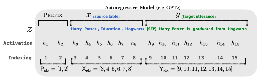
Prefix tuning is used to generate lightweight tuning of tasks. Prefix fine-tuning adds a continuous sequence of task specific vectors to the input, called a prefix. Different from prompt, prefix is completely composed of free parameters and does not correspond to the real token. Compared with traditional fine-tuning, prefix fine-tuning only optimizes the prefix. Therefore, we only need to store a copy of a large Transformer and a known task specific prefix, which will incur very little overhead for each additional task. Prefix Tuning improves the fine-tuning effect by adding a prefix to the data input to provide some prior knowledge to the model. The length of the prefix provided is an adjustable super parameter in training. In fine-tuning, it is also necessary to freeze the rest of the model and only train the super parameters related to the prefix.

The figure above shows the gpt2 model. The function of prefix is to guide the model to extract information related to x, so as to generate y better. For example, if we want to do a summary task, after fine tuning, we hope that prefix can guide the model to extract the core information in input x for summary. However, this will also lead to the increase of model input, increase of calculation amount and reasoning time, and the increase of prefix is difficult to ensure the training effect.

LoRA（Low-Rank Adaptation）

principle

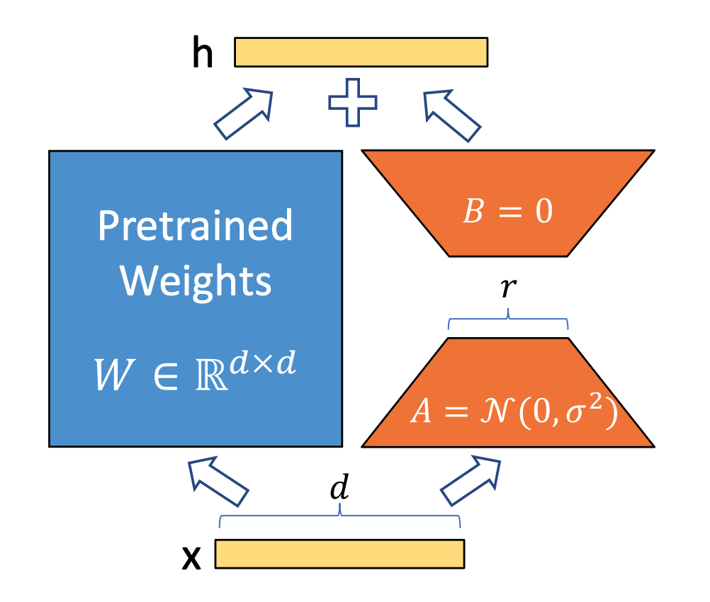
Because of the disadvantages of the above two methods, we hope to find a method that not only does not add additional inputs or change the model structure like full parameter tuning, but also can significantly reduce the amount of training parameters and reduce the cost of tuning. Based on this LoRA (Low Rank Adapter), it is the first to solve this problem. The following figure shows the overall architecture of LoRA. Lora adds a bypass beside the original weight matrix W, which is composed of two low rank matrices A and B. The combination of these two low rank matrices is used to approximate the Δ W increment matrix in the full parameter update. In the training process, we freeze the weight W of the original pre training model, and only update the two low rank parameter matrices A and B of LoRA. In order to ensure that the ability of the original model will not be affected after LoRA Adapter is added at the initial time of training, we use Gaussian initialization and zero initialization to initialize A and B respectively.

Assuming that the dimension of the original weight matrix is d × d, the dimension of LoRA low rank matrix A is set to r × d, and the dimension of matrix B is d × r, here we freeze the original weight, which is equivalent to updating only the incremental weight. It can be understood that we first conduct a dimension reduction operation through the A matrix, and then use the B matrix to conduct a dimension increase operation. In this way, the parameters of fine adjustment are reduced from the original d × d to 2 × d × r. Since the generally set parameter r will be far less than d, the amount of training parameters can be greatly reduced here. In the training process, because the pre training weight W is frozen, only the low rank matrices A and B are trained. Therefore, when saving the weight of LoRA training, only the low rank part with relatively small parameter amount needs to be saved. During training, GPU video memory usually stores the following contents: input data, model weight, intermediate results of the model, gradient and optimizer state. Compared with the full parameter fine-tuning method, the part of the input data in LoRA training remains unchanged. Because the original weight also needs to be involved in the calculation, the occupation of model weight and intermediate results is also unchanged (the increased LoRA part of the weight can be almost ignored). The analysis of video memory occupation of gradient is relatively complicated. Taking the gradient calculation of B in back-propagation as an example, the specific analysis is as follows:

h = W x + B A x = W m x ∂ B ∂ L = ∂ h ∂ L ∂ W m ∂ h ∂ B ∂ W m

Consider the first two terms of the B gradient. The dimension of the gradient is the same as the gradient of the pre training weight, which is d × d. However, because LoRA does not act on all layers of the model, and because of the reduction of training parameters, the storage of optimizer state is significantly reduced, because like the adam optimizer, it usually needs to store the first step degree and the second step momentum, and usually the values stored in the optimizer state are fp32 type values, so this part of video memory occupation is significantly reduced compared with full parameter fine-tuning, In general, the occupation of video memory is significantly reduced. In reasoning, the LoRA weight is combined with the original weight, that is, h=(W+BA) x, to get the same structure as the original model. This means that there is no need to change any structure of the model, and the reasoning parameters of the fine tuned model are exactly the same as those of the original model. And this way allows us to train different LoRA weights based on the same base model according to different business scenarios, and then load different LoRA weights on different applications. It is very flexible, and LoRA weights are usually very small and easy to store and load.

Summary of LoRA features:

• • Gaussian initialization for A and zero initialization for B;

• • The parameters of fine adjustment are reduced from the original d × d to 2 × d × r; r << d。

• • Reasoning does not increase any calculation, which is completely consistent with the original model architecture

• • Different lora models can be trained for loading in different scenarios based on the same base

experiment

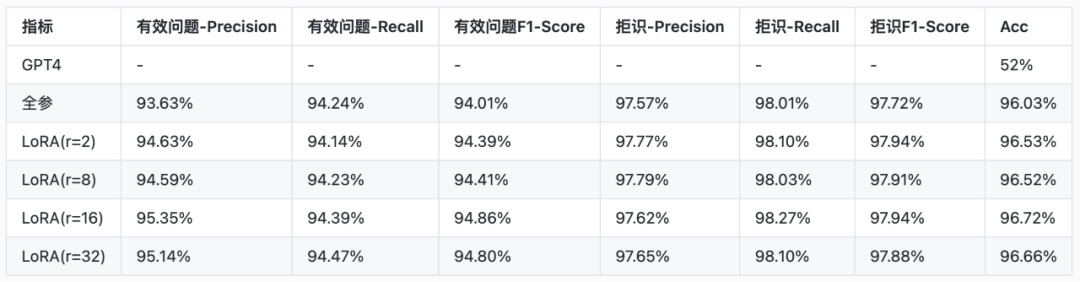
LoRA has been widely used in the industry for fine-tuning tasks in various scenarios, and has been verified to be effective and feasible in many tasks. We also carried out a single task fine-tuning practice based on two business scenarios. The principle of LoRA is that the increment matrix Δ W satisfies the low rank assumption, h = ( W + Δ W ) × x In Δ W It is indeed a low rank matrix. If this assumption is not met, then the decomposition of LoRA must have precision loss, and cannot achieve the best trimming effect. Therefore, it is necessary to select the appropriate r In theory, for complex tasks, larger r , but r The larger the value of, the larger the number of parameters that can be trained, and the training duration and video memory occupation will become larger at the same time. Generally speaking, increase r The value of will achieve better fine-tuning effect, but this is not necessarily the case. For simple tasks, fine-tuning too large training parameters will make the model training easy to over fit, resulting in poor effect. So in the experimental phase, we used two NLUs trade Business The data set compares full parameter training r At the same time, in order to prove the effect of fine-tuning, we also added GPT4 zero shot to compare the effect of this task. The experimental base model adopts qwen1.5-7b-base, and we compare the difference between full parameter fine tuning and LoRA r Fine tuning of and comparison of the effect of direct use of GPT4 ("effective problem" in business data set 2 refers to data labeled "other", and "rejection" refers to data labeled "other"):

NLU business Dataset 1:

NLU business Dataset 2:

From the experimental results of the two datasets in the table, we can see that in both scenarios, LoRA fine-tuning has achieved the same effect as full parameter fine-tuning. Especially in the second scenario, the effect of LoRA fine-tuning is actually better than full parameter fine-tuning. And from the experiment of the second business data set, the effect of LoRA fine tuning has a great relationship according to the selection of different ranks. The fine tuning effect first improves with the increase of rank, and achieves the best effect when the rank is 16, and then continues to increase without improving. Therefore, it is very important to select an appropriate rank value when using LoRA fine tuning.

QLoRA（ Quantized LoRA）

principle

Quantile quantization and block quantization

The main work of QLoRA is to further reduce the video memory occupation through model quantification. As can be seen from the introduction of the principle of LoRA above, LoRA fine tuning significantly reduces the video memory occupation of the optimizer's state part through a significant reduction of trainable parameters. In fact, the video memory occupation of model weights and intermediate variables does not change much. QLoRA reduces the size of the original semi precision model parameters by several times by defining the precision unit of NF4 and double quantization, thus further reducing the video memory occupation during training. Quantification essentially rounds a group of large data range numbers to a group of small data range numbers. For a simple example, we use 0-4 to represent the number of 0-9. Obviously, 0 corresponds to 0, 9 corresponds to 4, and 4 and 5 may both correspond to 2, which causes quantization error. Because 4 and 5 in the first type of data are mapped to 2 in the second type of data, which causes information loss, and this is the origin of quantization error. This error is irreversible, and many quantization methods are just to reduce this error as much as possible, but because of the reduction of data range, the error is actually inevitable. In order to reduce quantization errors as much as possible, QLoRA combines quantile quantization and block quantization techniques.

The idea of quantile quantification comes from probability distribution. Because the weight of the model usually conforms to the normal distribution, the quantization error can be effectively reduced by using this distribution feature. For example, at both ends of the distribution, due to the low probability of data occurrence, the mapping space can be expanded; In the middle of the distribution, the mapping space can be compressed due to the high probability of data occurrence. For example, if the original data type is 0-9 and conforms to the normal distribution, these data need to be represented by 0-4. In this case, the following mapping scheme can be adopted: mapping 0-3 to 0, 4 to 1, 5 to 2, 6 to 3, and 7-9 to 4. It can be seen that the number in the middle of the distribution is actually lossless quantization, and the quantization error is concentrated on both sides of the distribution. Due to the characteristics of normal distribution, the frequency of data on both sides is low, so this quantization method can effectively reduce the overall quantization error. The above examples are mainly used to help readers understand the basic principles of this quantitative method. In fact, in specific applications, it is necessary to use the cumulative distribution function in mathematics to determine the appropriate "quantile" point. Taking 4bit quantization as an example, there are 4 bit bits available for quantizing data, so 4bit quantization maps data into 16 numbers. The key to 4bit quantification is to find these 16 suitable quantiles, so as to ensure the efficient and accurate quantification process. 0 is usually of special significance for neural network weights, so we want to retain the position of 0 so that 0 can be mapped to the position of 0 after being quantized. Moreover, since the inverse function solution of the cumulative distribution function corresponding to 0 and 1 of the standard normal distribution is ∞ to − ∞, we need to provide an offset offset to reduce the range from [0,1] to [offset, 1-offset] 。 This is the main idea of quantile quantization. Let's briefly introduce the quantization process based on code.

 from  scipy.stats  import  norm
 import  torch

 def   create_normal_map (offset= zero point nine six seven seven zero eight three , use_extra_value= True ):

      if  use_extra_value:
          # one more positive value, this is an asymmetric type
         v1 = norm.ppf(torch.linspace(offset,  zero point five ,  nine )[:- one ]).tolist()  #Positive part
         v2 = [ zero ]*( sixteen - fifteen )  ## we have 15 non-zero values in this data type
         v3 = (-norm.ppf(torch.linspace(offset,  zero point five ,  eight )[:- one ])).tolist()  #Negative part
         v = v1 + v2 + v3
      else :
         v1 = norm.ppf(torch.linspace(offset,  zero point five ,  eight )[:- one ]).tolist()
         v2 = [ zero ]*( sixteen - fourteen )  ## we have 14 non-zero values in this data type
         v3 = (-norm.ppf(torch.linspace(offset,  zero point five ,  eight )[:- one ])).tolist()
         v = v1 + v2 + v3

     values = torch. Tensor(v)
     values = values.sort().values
     values /= values. max ()
      assert  values.numel() ==  two hundred and fifty-six
      return  values
   
   Q = create_normal_map()

Note the offset It may be slightly different from the above, but the purpose is to avoid obtaining − ∞ And + ∞ 。 use_extra_value Is to distinguish between symmetric quantization and asymmetric quantization. If use_extra_value For true Then there will be 7 values on the left side of 0, 8 values on the right side of 0, and a total of 16 values plus 0. And if use_extra_value For false , there are 7 values on the left and right of 0, and 0 accounts for 2 values. The code logic is as follows: torch.linspace Evenly get offset 8 numbers to 0.5. (Why is it 0.5? Because of the standard normal distribution, the cumulative distribution probability corresponding to position 0 is 0.5). Then through scipy.stats Packaged norm.ppf Methods The quantile value of the corresponding point was obtained, and then the 0 corresponding to the 0 position was added. After normalization, 16 quantiles of 4-bit quantization were obtained.

Block quantization, its idea is to divide the data before quantization into several blocks, and the data of each block is quantized in each block, so as to reduce the influence of outliers in the whole data on the quantization effect as far as possible. Each quantized block records its own quantized constant. The quantized constant is calculated as the maximum value of the data in the block, because it is necessary to calculate the normalized value based on the quantized constant, and then obtain the quantized value according to the quantile index closest to the value. During inverse quantization, it is only necessary to find the quantile based on the index value, and then multiply the corresponding quantization constant to obtain the inverse quantization result.

Dual quantization and paging optimization

As mentioned in quantile quantization and block quantization above, the model needs to save not only the quantized results, but also the quantized constants of each block, and the quantized constants are usually full precision or half precision, that is, 32-bit or 16 bit. The double quantization of QLoRA is to quantize the quantization constant by 8bit again. When quantizing the quantization constant, QLoRA will quantize every 256 quantization constants as a group. Because double quantization is used, we also need to reverse quantization twice to restore the quantized value. Finally, paging optimization is a further optimization for gradient checkpoints to prevent video memory OOM problems when video memory usage peaks. QLoRA paging optimization is actually to transfer part of the saved gradient checkpoints to the CPU memory when the video memory is insufficient, which is the same as transferring the computer's memory data to the conventional memory paging on the hard disk. The content of gradient checkpoints is not the focus of this article, so it will not be explained here. Combined with quantile quantization, block quantization, double quantization and paging optimization, QLoRA achieves extremely low video memory occupancy fine tuning, and can achieve almost no loss of fine tuning accuracy compared with the original LoRA. Even compared with full parameter fine tuning, many works have proved that the precision loss of QLoRA is very small, and it is also widely used in fine tuning of many scenes in the industry.

experiment

NLU business Dataset 1: Conduct QLoRA training for Qwen 1.5-7B on an A800, use the same dataset to train 5400 steps, enable gradient_checkpointing, and insert lora adapters in all linear layers. The results show that QLoRA significantly reduces the video memory occupation, and there is almost no performance degradation compared with the original LoRA tuning. However, because QLoRA requires additional quantization and inverse quantization time, the training time will be slightly longer than the ordinary LoRA.

AdaLoRA（Adaptive Low Rank Adaptor）

principle

It was mentioned in the introduction of LoRA (Low rank Adapted) that by adding a low rank adapter bypass, LoRA greatly reduces the amount of tuning parameters and video memory occupation. However, the setting of the super parameter (r) in LoRA is globally unified, that is, the same rank is used in all modules. This method obviously cannot meet the weight increment of different modules Δ W Actual situation with different ranks. Therefore, from a theoretical perspective, it is more reasonable to set different ranks according to the importance of different modules in the model. In order to solve this problem, AdaLoRA (Adaptive Low Rank Adapter) proposed a method to adaptively adjust the rank of each module. Specifically, AdaLoRA updates Δ W parametrically based on singular value decomposition (SVD). Through this SVD based method, AdaLoRA can efficiently cut out unimportant singular values without complex SVD calculation, thus reducing the amount of calculation to achieve the purpose of efficient fine tuning. SVD (Singular Value Decomposition) is an important algorithm of traditional machine learning, which can be used in matrix decomposition. One of the most important properties of SVD decomposition is that it can approximate the original matrix through the first k singular values and their corresponding left and right singular vectors, so it is often used in dimension reduction algorithms. SVD decomposition can be expressed as

A = U Σ V T

Where 𝑈 and 𝑉 are both unitary matrices, that is

U T U = I V T V = I

The unitary matrix is the generalization of orthogonal matrix on complex number. 𝛴 is the singular matrix of 𝐴, which is a diagonal matrix. The value on the diagonal is the singular value of the matrix 𝐴. Because different modules have different contributions in a model, it will bring many benefits if different ranks can be assigned to different modules according to their importance when using LoRA. First of all, assigning smaller ranks to modules with lower importance will effectively reduce the computation of the model. Secondly, if more important features can be assigned a larger rank, then the details of features can be captured more effectively. This is the motivation of AdaLoRA. To achieve this goal, the following problems need to be solved:

1. 1. How to integrate SVD and LoRA?

2. 2. How to model the importance of parameters?

3. 3. How to automatically calculate the value of (r) according to its importance?

Integrating SVD and LoRA

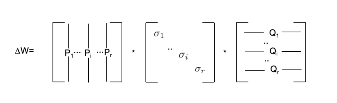
AdaLoRA replaces the binomial of LoRA with the trinomial of SVD. AdaLoRA is calculated as follows:

W = W + Δ W = W + P Λ Q

Including P And Q Are orthogonal matrices Λ Is a diagonal matrix. In this way, the structure of LoRA is perfectly transformed into the form of three terms in SVD decomposition. In order to make the three terms of the decomposition truly meet the properties of SVD decomposition, AdaLoRA adds a pair of P And Q Constraints of P And Q Meet the property of orthogonal matrix.

R ( P , Q ) = ∣ P T P − I ∣ F two + ∣ Q Q T − I ∣ F two

Including I Represents the identity matrix. And because P  、  Q Intermediate Λ It is a diagonal matrix, so you can use vectors to save space. The following code example is the AdaLoRA implementation of the PEFT library, which clearly shows the structure of the AdaLoRA layer:

 self.lora_A[adapter_name] = nn. Parameter(torch.randn(r, self.in_features))
 # Singular values
 self.lora_E[adapter_name] = nn. Parameter(torch.randn(r,  one ))
 # Left singular vectors
 self.lora_B[adapter_name] = nn. Parameter(torch.randn(self.out_features, r))

In code r Is a predefined super parameter, that is, the initial r , following the one in LoRA r It means matrix A The dimension of is r × d  ， E A matrix is a r × one This represents the diagonal matrix in SVD decomposition, B The dimension of is d × r  。

The following code block shows AdaLoRA in loss Add restriction code for orthogonal matrix in. You can see that AdaLoRA loss Added p p T − I The Fro norm of, minimize the loss Can make p p T It is close to the identity matrix and satisfies the orthogonal property of SVD decomposition. According to the model structure and loss function design described above, SVD decomposition is perfectly combined with LoRA low rank decomposition.

 for  n, p  in  self.model.named_parameters():
      if  ( "lora_A"   in  n  or   "lora_B"   in  n)  and  self.trainable_adapter_name  in  n:
         para_cov = p @ p. T  if   "lora_A"   in  n  else  p. T @ p
         I = torch.eye(*para_cov.size(), out=torch.empty_like(para_cov))
         I.requires_grad =  False
         num_param +=  one
         regu_loss += torch.norm(para_cov - I, p= "fro" )
 if  num_param >  zero :
     regu_loss = regu_loss / num_param
 else :
     regu_loss =  zero
 outputs.loss += orth_reg_weight * regu_loss

Calculation parameter importance

In AdaLoRA, we combine LoRA low rank decomposition with SVD decomposition, and the form of decomposition is P ∧ Q, as shown in the figure below. Based on this, we can leave the triplet with high importance and discard the triplet with low importance according to the triplet composed of singular vectors in P and Q matrices and singular values in Λ. Set the r of each module by setting the low importance triplet to 0, which achieves the original purpose of AdaLoRA and solves the problem that all modules in LoRA have the same rank.

The importance score is calculated from sensitivity and uncertainty. When calculating sensitivity, for a single parameter, the product of the weight of the parameter and its absolute gradient value is used as the sensitivity value. Since the weight and gradient are the values in the current batch data during training, which may have large differences between different batches, the sliding average operation is applied to them, and the sliding average value during the whole training process is recorded as the sensitivity score. In addition, it is also necessary to calculate the uncertainty score to measure the fluctuation of the sensitivity of parameters in the training process. The uncertainty score at a certain time is obtained by subtracting the moving average value of the sensitivity score at that time from the sensitivity score at that time to evaluate the parameter change amplitude. Finally, the moving average operation is also applied to the uncertainty score to obtain the final uncertainty score. The following are some fragments of relevant key code.

 def   update_ipt (self, model):
      # Update the sensitivity and uncertainty for every weight
      for  n, p  in  model.named_parameters():
          if   "lora_"   in  n  and  self.adapter_name  in  n:
              if  n  not   in  self.ipt:
                 self.ipt[n] = torch.zeros_like(p)
                 self.exp_avg_ipt[n] = torch.zeros_like(p)
                 self.exp_avg_unc[n] = torch.zeros_like(p)
          with  torch.no_grad():
             self.ipt[n] = (p * p.grad). abs ().detach()
              # Sensitivity smoothing
             self.exp_avg_ipt[n] = self.beta1 * self.exp_avg_ipt[n] + ( one  - self.beta1) * self.ipt[n]
              # Uncertainty quantification
             self.exp_avg_unc[n] = (
             self.beta2 * self.exp_avg_unc[n] + ( one  - self.beta2) * (self.ipt[n] - self.exp_avg_ipt[n]). abs ()
             )

Finally, the product of sensitivity score and uncertainty score is used to express the importance score of the parameter. For triples P i  ，  σ i  ，  Q i For example, the importance score of a triple is equal to the weighted sum of the three values of the triple.

 def   _element_score (self, n):
      return  self.exp_avg_ipt[n] * self.exp_avg_unc[n]

Automatically calculate the value of rank 𝑟 according to the importance

After obtaining the importance scores of each pair of triples in AdaLoRA, you can determine the importance scores of each module r Value. In singular value decomposition (SVD), the importance of a feature depends on the absolute value of its corresponding singular value. Based on this idea, AdaLoRA adopts a pruning strategy, namely Λ Medium λ Set the unimportant element to 0, and use the Λ k ( t ) To replace. Since this strategy does not involve the modification of matrix size Λ Always keep r × r Size of. In the super parameter of AdaLoRA, the initial rank needs to be defined ini t r And final rank t a r g e t r  。 In training, the model will gradually keep only the triples with high importance according to the importance score of the triples, and set the unimportant ones to 0. In this way, the initial rank will eventually be reduced to the final rank. However, the rank of AdaLoRA modules in each layer of the model r Values are not necessarily reduced to the final rank. For example, if you add AdaLoRA adapters to 10 layers of the model, and set the initial rank to 16 and the final rank to 8, the total number of initial triples is ten × sixteen = one hundred and sixty  。 During the training process, the former will be retained according to the importance score of each triple ten × eight = eighty (The remaining 80 triples are set to 0). The key codes are as follows:

 all_score = []
 #Get the importance score of each triple
 # Calculate the score for each triplet
 for  name_m  in  vector_ipt:
     ipt_E = value_ipt[name_m]
     ipt_AB = torch.cat(vector_ipt[name_m], dim= one )
      # 
     sum_ipt = self._ combine_ipt(ipt_E, ipt_AB)
     name_E = name_m %  "lora_E"
     triplet_ipt[name_E] = sum_ipt.view(- one ,  one )
     all_score.append(sum_ipt.view(- one ))

 #Take the score of the number of previous widgets as the threshold value of the mask
 # Get the threshold by ranking ipt
 mask_threshold = torch.kthvalue(
 torch.cat(all_score),
 k=self.init_bgt - budget,
 )[ zero ].item()

 rank_pattern = {}
 #Set the triplet less than threshold value to 0 directly
 # Mask the unimportant triplets
 with  torch.no_grad():
      for  n, p  in  model.named_parameters():
          if   f"lora_E. {self.adapter_name} "   in  n:
             p.masked_fill_(triplet_ipt[n] <= mask_threshold,  zero )
             rank_pattern[n] = (~(triplet_ipt[n] <= mask_threshold)).view(- one ).tolist()
 return  rank_pattern

So far, the basic principles of AdaLoRA have been fully introduced. The next question to be discussed is how to determine how many triples need to be retained at the current training time, and how many triples need to be lost by the mask, that is, how to determine the value of the widget in the above code. In fact, a warm up mechanism similar to deep learning is used here. The following is the specific process of calculating the budget. Two super parameters of AdaLoRA are required: t ini t And t f ina l  。 The meaning of these two super parameters is the number of training steps. Specifically, before t ini t In step, AdaLoRA uses the initial rank ini t r That is, the rank of the matrix is not changed, so that the model can achieve a relatively stable effect in the early stage; At the end of t f ina l In step, the rank of AdaLoRA is equal to the set final rank t a r g e t r  。 For the number of training steps in the middle, make the budget value from the initial value with a cubic amplitude ini t r Gradually reduce to the target value t a r g e t r  。

 def   budget_schedule (self, step:  int ):
     tinit = self.peft_config.tinit
     tfinal = self.peft_config.tfinal
     total_step = self.peft_config.total_step
      # Initial warmup
      if  step <= tinit:
         budget = self.init_bgt
         mask_ind =  False
      # Final fine-tuning
      elif  step > total_step - tfinal:
         budget = self.target_bgt
         mask_ind =  True
      else :
          # Budget decreasing with a cubic scheduler
         mul_coeff =  one  - (step - tinit) / (total_step - tfinal - tinit)
         budget =  int ((self.init_bgt - self.target_bgt) * (mul_coeff** three ) + self.target_bgt)
         mask_ind =  True   if  step % self.peft_config.deltaT ==  zero   else   False
      return  budget, mask_ind

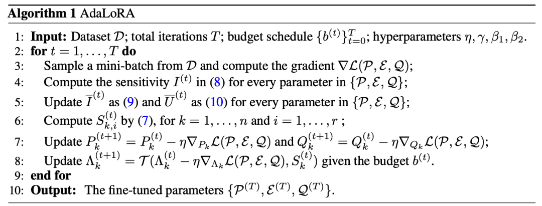
AdaLoRA has more formula derivation and calculation logic than LoRA, which is complex to introduce. Its process can be summarized by the following flow chart in the original paper

• • Line 1: Determine the super parameters involved in the dataset and AdaLoRA;

• • Lines 2-9: the training process of the model, and the total number of training steps is 𝑇;

• • Line 3: Calculate the gradient of the feature based on the loss;

• • Line 4: Calculate the sensitivity of the characteristics;

• • Line 5: calculation of slip values for sensitivity and uncertainty;

• • Line 6: Calculate the importance of the entire triple according to sensitivity and uncertainty;

• • Line 7: Update the values of P and Q according to the conventional gradient descent;

• • Line 8: Use the strategy of setting 0 when the threshold value is lower than to update Λ

• 
  

experiment

Use AdaLoRA to train. The places that need to be changed in the trainer script of the transformers library are

• • Set the total steps of the workout

 if  self.rankallocator  is   not   None : 
     self.rankallocator.set_total_step(max_steps)

• • After each optimizer.step, calculate the importance of the triple (left singular vector, right singular vector and singular value), get the rank r budget budget according to the current step, and then set 0 according to the importance and budget.

 optimizer.step()
 lr_scheduler.step()
 # Update the importance of low-rank matrices
 # and allocate the budget accordingly.
 model.base_model.update_and_allocate(global_step)

experimental result

We are at NLU business Data set 1 also compared the effects of AdaLoRA and LoRA tuning based on the qwen1.5-7B model, tried several sets of super parameter experiments, and failed to achieve good results. Compared with LoRA tuning, there is a certain performance gap in this scenario (the best result that has been tried in setting the r value of adalora given in the table). Based on the experimental results, we suspect that AdaLoRA's positive definite hypothesis is a bit too strict. Adding such strict settings to the loss function may limit the effect of the model. However, AdaLoRA is very valuable for the idea of changing the rank of different modules, and there are still many high-quality work based on this idea in the future.

NLU business Dataset 1:

SoRA（Sparse low rank adaptation）

principle

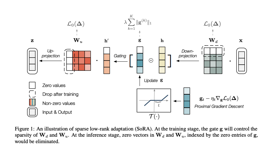
In the previous article, the efficient tuning methods of LoRA and AdaLoRA have been introduced in detail. Although LoRA shows excellent performance, the rank of each module is fixed and unchangeable, which may not be ideal in some application scenarios. In contrast, AdaLoRA solves this problem by pruning based on the importance of parameters to give different modules different ranks. However, the assumption of this method is relatively strict, because it adds strict restrictions on orthogonality to the loss function, which may affect the model effect to a certain extent. For this reason, SoRA proposed an innovative method of dynamically adjusting rank. In the training phase, SoRA controls the rank under the sparsity of the gate by introducing the gate unit optimized based on the near end gradient method. In the reasoning phase, this method reduces each SoRA module back to a simple but excellent LoRA module by eliminating the parameters corresponding to the zeroed rank, thus improving the flexibility and adaptability while ensuring the efficiency of the model. The figure below is the schematic diagram of SoRA structure in the paper:

SoRA adds a gate element to the low rank decomposition of ordinary LoRA g , as can be seen in the figure, enter X After a dimension reduction matrix W d , become h , and then through the door unit g Control W d (the operation of the control rank lies in the gate unit g Some values are 0), similar to putting W d The operation is adaptive compared with adalora, that is, there is no need to manually set the target r budget and set it to 0 according to the threshold. The update function of the gate operation is as follows: (The reason for this setting is that it is the analytic solution to the LASSO problem of the near end gradient descent algorithm: the soft threshold function)

g t + one ← T ( g t , λ )

among

T λ ( x ) := ⎩ ⎨ ⎧ x − λ , zero , x + λ , x > λ − λ < x ≤ λ x ≤ − λ

The structure code of SoRA module is as follows:

 def   init (self, ...):
     ...   #Omission
      if  r >  zero :
         self.lora_A = nn. Parameter(weight.new_zeros((r, in_features)))
         self.lora_B = nn. Parameter(weight.new_zeros((out_features, r)))
         self.gate = nn. Parameter(torch.randn( one , r))
         self.scaling = self.lora_alpha / self. r
         nn.init.kaiming_uniform_(self.lora_A, a=math.sqrt( five ))
         nn.init.zeros_(self.lora_B)

 def   forward (self, x):
      return  ((self.lora_dropout(x) @ self.lora_A.T).mul(self.gate) @ self.lora_B.T) * self.scaling

Moreover, the operation of updating the gate value mentioned above is performed in the step function optimized by the optimizer, because the gate parameter does not need to be updated through the traditional gradient descent. The key code fragments are extracted as follows, where sparse_lambda is a super parameter.

 #P.data represents the value of gate sparse_lambda is a super parameter
 if  self.sparse_lambda >  zero :
     p.data[p.data > self.sparse_lambda] -= self.sparse_lambda
     p.data[p.data < -self.sparse_lambda] += self.sparse_lambda
     p.data[ abs (p.data) < self.sparse_lambda] =  zero

This completes the function of updating the gate unit parameters described above. In addition, we need to add the loss of the spark gate unit to the loss, which is equal to the 1 norm of the gate parameter. This is due to the need of solving the near end gradient descent algorithm. The key codes are as follows:

 if  self.args.train_sparse:
     sparse_loss =  zero
     p_total =  zero
      for  n, p  in  model.named_parameters():
          if   "lora.gate"   in  n:
             sparse_loss += torch. sum (torch. abs (p))
             p_total += torch.numel(p.data)  
     loss += self.sparse_lambda * sparse_loss / p_total

experiment

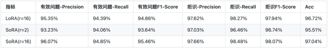
We are in two NLUs business Based on the qwen1.5-7B model, we compared the effects of SoRA, AdaLoRA and LoRA fine-tuning on the dataset, and tried several sets of super parameter experiments. The experimental results show that SoRA fine-tuning has good effects in both business scenarios. Especially in the second business scenario, each indicator achieved the best results.

NLU business Dataset 1:

NLU business Dataset 2:

Fine tuning acceleration practice

Several efficient low parameter fine-tuning methods have been introduced previously, which can effectively save training resources and speed up training in fine-tuning tasks. High efficiency fine-tuning can save video memory and computation by using low parameter fine-tuning strategy, and can also speed up training by optimizing the training process. Combining these two methods can make the fine-tuning training task more efficient, and observe the fine-tuning effect more quickly on the premise of saving training resources. The following will share relevant practical attempts to use the large model training acceleration tool Unslow to carry out acceleration experiments.

Unsloth

Unslow accelerates training by using optimized backpropagation modules to cover some modules of large model modeling. In this process, the original PyTorch module is rewritten with the Triton kernel by manually implementing the backpropagation step. Unslot can not only reduce memory usage, but also speed up fine tuning. Compared with conventional LoRA or QLoRA, the precision is reduced to 0%. Specifically, Unslot uses OpenAI's Triton language to rewrite the forward and backward propagation methods of such structures as RoPE, MLP, and LayerNorms, which optimizes the computing performance and video memory occupation of the GPU. Because modern large-scale language models usually have very deep structures, such as LLaMA, which usually contains 32 or more levels, it is necessary to calculate the derivatives of a large number of parameters as intermediate variables in the back-propagation process, and to perform very deep chain derivatives. During LoRA fine-tuning, the dimensions of the LoRA layer may range from 8 to 128, but the dimensions of the LLaMA structure are usually multiples of 1024, or even 4096. The core of the Unslow acceleration mechanism is to optimize the chain matrix derivation calculation with large dimensional changes, and widely use the inplace operation in the gradient calculation and update process, so as to further reduce the video memory occupation.

Fine adjustment acceleration

• • Support the acceleration of models llama, gemma, deepseek, and qwen.

• • Unslot is based on the bisandbytes package. It only supports the lora mode and its variants in the peft library, and supports qlora.

• • The accuracy loss is 0, and the acceleration is completely lossless.

• • Pretrain is not supported

• • Open source version only supports single card, not multiple cards

• • Models that do not support moe structure

The change method is as follows: use the FastLanguageModel.get_peft_model method of the FastLanguageModel of the slot package to replace the get_peft_model method of the peft package.

 from  unsloth  import  FastLanguageModel

 if  model_args.use_unsloth:
      from  unsloth  import  FastLanguageModel   # type: ignore

     unsloth_peft_kwargs = {
          "model" : model,
          "max_seq_length" : model_args.model_max_length,
          "use_gradient_checkpointing" :  "unsloth" ,
     }
     model = FastLanguageModel.get_peft_model(**peft_kwargs, **unsloth_peft_kwargs)
     
 else :
     lora_config = LoraConfig(
         task_type=TaskType. CAUSAL_LM,
         inference_mode= False ,
         use_dora=finetuning_args.use_dora,
         **peft_kwargs,
     )
     model = get_peft_model(model, lora_config)

test result

At present, the test results show that under qwen 1.5 and llama3, there are obvious training acceleration and video memory occupancy reduction effects. We used an A800 to test the acceleration effect under the lora fine-tuning of the two scenes. The qwen and llama series can effectively reduce the training duration by about 30%, increase the training speed by about 40%, and reduce video memory occupancy by 40%+. If the 4bit qlora fine tuning is used, the video memory occupation can be further reduced to a very low level.

NLU business Dataset 2:

(Note: because the data set is large and the training time is long, the training duration is the total training duration estimated according to the training duration of the first 1000 steps, which may be slightly different from the actual total training duration.)

NLU business data Set 1: The test results of 7412 data trainings, 3 epochs, 4 batch_size, and 5559 steps are as follows (complete training parameters are attached at the end):

• •  Training acceleration effect comparison
  Model ：qwen1.5-7b / llama3-8b / qwen1.5-14b

Acceleration method: none refers to the trainer of the native transformers library, excluding other acceleration methods/enable flash atten tion/enable idle/enable flash atten ion and idle at the same time

• • Comparison of the effect of reducing video memory occupation:

summary

This paper introduces the principle analysis and experimental results comparison of several efficient fine-tuning methods in detail, and makes some practical attempts to speed up fine-tuning based on Unslot. The experimental results show that the combination of excellent low parameter fine-tuning methods and fine-tuning acceleration can achieve extremely efficient fine-tuning of large models, and can achieve the effect comparable to full parameter fine-tuning at a very low resource occupation.

About the author: Liu Hui, algorithm engineer of 58 local TEG-AILab big language model, is mainly responsible for SFT fine-tuning of Lingxi big language model.

reference

[1] Houlsby N, Giurgiu A, Jastrzebski S, et al. Parameter-efficient transfer learning for NLP [ C ] //International conference on machine learning. PMLR, 2019: 2790-2799.  

[2] Li X L, Liang P. Prefix-tuning: Optimizing continuous prompts for generation [ J ] . arXiv preprint arXiv:2101.00190, 2021.

[3] Hu E J, Shen Y, Wallis P, et al. Lora: Low-rank adaptation of large language models[J]. arXiv preprint arXiv:2106.09685, 2021.

[4] Dettmers T, Pagnoni A, Holtzman A, et al. Qlora: Efficient finetuning of quantized llms [ J ] . Advances in Neural Information Processing Systems, 2024, 36.

[5] Zhang Q, Chen M, Bukharin A, et al. Adaptive budget allocation for parameter-efficient fine-tuning [ C ] //International Conference on Learning Representations. Openreview, 2023.

[6] Ding N, Lv X, Wang Q, et al. Sparse low-rank adaptation of pre-trained language models [ J ] . arXiv preprint arXiv:2311.11696, 2023.

[7] https://github.com/huggingface/peft

Department Introduction

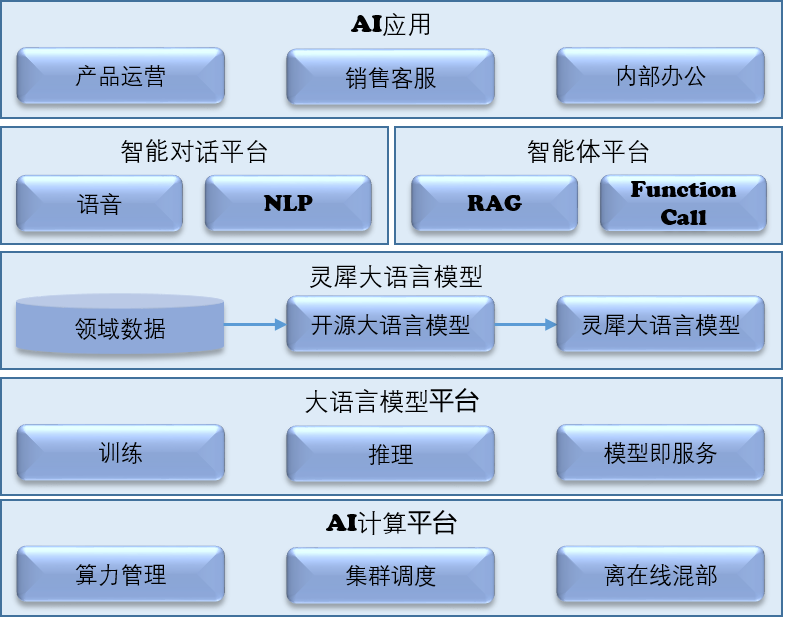
58 The AI Lab in the same city belongs to the TEG technology engineering platform group, which aims to build an AI platform with leading models, agility and ease of use, and help AI applications to be widely implemented in the company. At present, the department has built a large vertical model of 58 local life service fields (recruitment, real estate, cars, local services) - Lingxi big language model ChatLing, and created AI computing platform, big language model platform, AI agent platform, intelligent dialogue platform and other products and capabilities.