How to use SPSS for time series analysis?

Latest answers Change
Q: Will the tempered glass fall when it bursts
What is the access to the nuclear hole 2020-06-24
R How to reverse when blocking in front 2020-06-29
Difference between mallard duck and common duck 2020-07-01
Do you want the beef soaked in blood 2021-12-10
Related recommendations

What is the hearing distance of human ear
How to cancel a credit card

Can I eat things smoked with sulfur

What does it mean that everything is fate

What material is pvc oil

How old can I get a marriage certificate
How to check the express without express number

How long does it take to cook or steam dumplings
Is cicada a pest or a beneficial insect
How many days of pregnancy can be measured by ovulation test paper

What does 9921 mean

All very good. Did you remarry tomorrow
How to keep garlic cloves