There are two possible ways to combine sales rate and sales area data into a chart.The detailed operation steps are as follows: Method 1: Make the required data in the form of conventional tables, and add the two kinds of data to the same chart.First, arrange the sales rate data into tables as required.Then, add the sales area data to the table, and select the appropriate chart type (such as the disconnection chart) for presentation.Next, right click the chart, select "Change" in the pop-up menu, and enter the selected type of wire removal chart. Method 2: Make the sales rate and sales area into the required chart form, and unify the coordinate axis.First, arrange the sales rate data into the required format, and make the required line chart or other types.Secondly, similarly, arrange the sales area data into the required format, and make it into the required polylines or scattered points and other types.Then, set the same coordinate system between the two layers, and ensure that one layer (without background fill color) is placed above to cover the other layer. Through one of the above two methods, you can combine the sales rate and sales area into a chart.However, in the case of large data differences, how to better display the chart content may become a challenge. Conclusion: The above two methods can combine the sales rate and sales area into a chart, but it is the key to choose the appropriate method according to the specific situation.If the data is quite different, you may need to further adjust the chart type or add other elements to improve readability.
Change the form of the table as follows: the top row B2 to the right is the date, 11.12, 11.13, etc., A2 is A, enter the value backward: 24.72%, enter the value to the right in turn, and enter the value of B in the same way, select the area, and turn into a line chart.
First make a column chart, then select the group of columns you want to turn into a polyline, right click, change the series icon type, polyline chart, OK
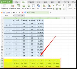
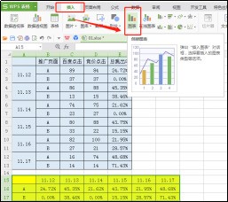
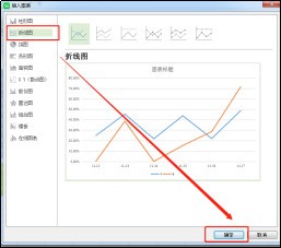
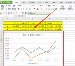
1. Open the Excel table, extract two groups of data and sort them out. 2. Click the left mouse button to expand and select the sorted data, click "Insert" above, find "Chart", and click to enter. 3. On the chart page, find the "Line Chart", select the corresponding line chart, and then click OK. 4. Click the chart title to make changes. At this time, the production of the line chart is completed.